Reversible Automata / Irreversible Automata
Chapters:
Acknowledgements
Introduction
CAs & You
The Mechanism
Conclusions
Bibliography
Media:
Images
Video
Resources:
PDF
Source Code
Acknowledgements
Introduction
CAs & You
The Mechanism
Conclusions
Bibliography
Media:
Images
Video
Resources:
Source Code
Reversible Automata / Irreversible Automata
A Catalog of the Creative Project
Presented to
The Faculty of the School of Art and Design
San Jose State University
In Partial Fulfillment
of the Requirements for the Degree
Master of Fine Arts
By
John Bruneau
November 2005
A Catalog of the Creative Project
Presented to
The Faculty of the School of Art and Design
San Jose State University
In Partial Fulfillment
of the Requirements for the Degree
Master of Fine Arts
By
John Bruneau
November 2005
I would like to thank my parents, Henry and Sue Bruneau, for helping me get through the rough early days I endured in our public education system. Oh yeah, and Life. I would like to thank my committee, Joel Slayton, Shannon Wright, and Steve Durie, for all the advice and support they have given me, even if they weren’t sure what exactly it was I was doing sometimes. This goes for my parents as well. I would like to thank Mike Hayward for first introducing me to the world of Cellular Automata and Artificial Life. I would like to thank Rudy Rucker for rekindling the fascination as well as the wealth of information and inspiration he provided. I would like to thank all my friends, those who soldered and those who helped out in a pinch when it was the final hour, Ethan Miller, Sheau Ching Lee, Michael Weisert, Thomas Asmuth, Vera Fainshtein, and Bruce Gardner. If I missed anyone I’m sorry I was kind of delirious. I would especially like to thank Kyungwha Lee, without her effort and support I would have accomplished nothing on time if at all. I would also like to thank the unknown for keeping me curious.
TABLE OF CONTENTS
| I. | INTRODUCTION | |
| II. | CELLULAR AUTOMATA AND YOU | |
| III. | THE MECHANISM | |
| IV. | CONCLUSIONS | |
| V. | BIBLIOGRAPHY |
“If only I could move through time as freely as I can move through space.” – This thought has been especially prevalent in my mind throughout my years in graduate school. I felt it was only fitting that my graduate thesis evolve out of it. There is much conjecture about time manipulation, the possibilities, the impossibilities and the paradoxes. I wanted to find a system that was not bound by time in the same manner we are. That system came in the form of reversible Cellular Automata. Cellular Automata (CAs) are simple graphic self-generating mathematical algorithms. These algorithms exhibit emergent, even lifelike, behavior, which can be very complex even when the rules they follow are quite simple. Reversible Cellular Automata follow rules such that taking a step forward in time is as simple as taking a step back. The Irreversible Automata in this piece are you and I. If you are a researcher in the field of Artificial Life, or a subscriber to the philosophy of Universal Automatism this is not an unusual assumption. The other assumption I make is that we are in fact trapped in a forward-moving linear chronology. Besides the strictly philosophical arguments, there exist some conjectures in quantum mechanics about the breaking of causality when it comes to entanglement and “spooky action at a distance”. In my macro-world, day to day struggle, however, time-does-exist as an unbreakable restraint.
The basis for the work is these two opposing systems. One system unbound by time, and the other (the one I live in) bound by time. The question now was: How do these two systems really function? The answer to this problem came in Joel Slayton’s foreword to Media Ecologies by Mathew Fuller:
“...to discover or reveal the determinates of any complex system is to collide it with another.”
I thus began developing a mechanism for colliding these two systems together. What would happen to causality if such a collision were to occur? Could causality, at least in concept, be bent or broken? I needed the resulting project to be an environment where the underlying computation of each system was exposed to the computation of the other. Opening people to CAs is one issue, but opening CAs to people is another. For the human element to absorb the computation of the cellular automata, we had to want to absorb it. The environment needed to present the CAs in an engaging and aesthetic incarnation. Cellular Automata cannot be enticed to absorb a foreign computation in the same way that we can. I had to expose their innards to the air. Using an elaborate system, I extracted key elements of their algorithms from the inner workings of the computer, the black box they normally reside in. Using a monitor, camera and 192 LEDs I opened up the Cellular Automata algorithm to the natural world in such a way that we human computations were able to freely inhabit it. Both systems now occupied a single reality.- Slayton Media Ecologies p. ix

...the key point is that even though their underlying rules are really simple, systems like cellular automata can end up doing all sorts of complicated things -- things completely beyond what one can foresee by looking at their rules and things that often turn out to be very much like what we see in nature.
– Wolfram Hal’s Legacy: 15 p7
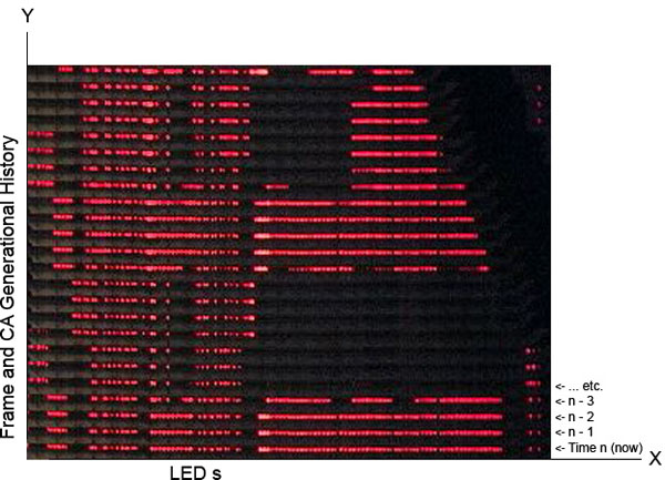
The discipline of Artificial Life is determined to make up for the shortcomings of Artificial Intelligence by using simple rules to model complex lifelike behavior. Cellular Automata are one of the simplest forms of self-replicating systems in ALife. CAs visually exist as a grid of changing cells. Each cell in the grid reacts based on the cells around it, hence the term Cellular Automata. The simplest form of nontrivial Cellular Automata are binary, one-dimensional, and have a neighborhood consisting of only three cells. Binary refers to the fact that each cell only has two states; it is either on or off, dead or alive. One-dimensional means that calculations aren’t applied to a multi-dimensional matrix, but only a list, a single row. In graphing one-dimensional CAs, the Y-axis represents history. Every new generation appears as the bottom line while the previous generations scroll upward. A three-cell neighborhood consists of the cell itself, the cell to its left and the cell to its right. For each successive generation to be calculated, a rule is applied to every cell in the generation before it. The rule determines whether a cell in the next generation will be on or off based on the states of the cells in its neighborhood. In this system of binary, 1D, three-cell neighborhood CAs, each neighborhood will be in one of eight possible configurations. A rule lays out whether a cell will be on or off in the next generation based on which one of these configurations matches its own neighborhood. This results in 2^8 or 256 possible rules.
In his book, A New Kind of Science, the mathematician Steven Wolfram has categorized the patterns that that these rules generate into four classes:
Class 1: Static, dead, no change
Class 2: periodic, repetitive
Class 3: chaotic, random
Class 4: deterministic, neither completely random nor repetitive
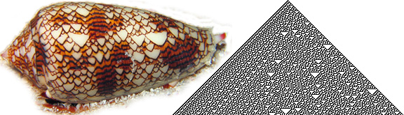
Cone Snail, Photographer: Richard Ling
Cellular Automata Rule 30
The patterns that most rules generate tend to die out or become periodic. Wolfram’s Class 3 rule 30 works as a random number generator. But there are rules such as Wolfram’s rule 110 that produce Class 4 patters, rich computations which the computer scientist Rudy Rucker refers to as “Gnarly”. Computational structures continue to evolve and interact in ways that cannot be predicted by any mathematic shortcut. The new generation can only be determined from the previous generation. These characteristics are not limited to one-dimensional Cellular Automata; John Conway’s Game of Life, the wave equation, and pattern formation in nature all produce Class 4 computational structures. Matthew Cook, Wolfram’s research assistant, was even able to prove that rule 110 was computation universal. A universal computation is able to emulate any other computation. There are many universal computations, but this one is surprisingly simple. Rule 110 is written out as 01101110, a mere eight digit binary number. This demonstrates a significant parallel to naturally occurring physical systems. Wolfram even goes so far as to suggest that nature itself is a universal computation.
Now here's the good bit: it turns out that those simple computer programs (Cellular Automata) can often behave like universal computers. And what that means is that they can do stuff that's as complicated as anything, including anything our fancy electronic computers do. There's a major new piece of intuition here. You see, people have tended to assume that to make a universal computer -- a general-purpose machine -- the thing had to be constructed in a pretty complicated way. Nobody expected to find a naturally occurring universal computer lying around. Well, that's the thing I've found that isn't true. There are very simple universal computers. In fact, I think that lots of systems we find all over the place in nature can act as universal computer.
.[W]e can think of the behavior of any system in nature as being like a computation: the system starts off in some state -- that's the input -- then does its thing for a while, then ends up in some final state, which corresponds to the output. When a fluid flows around an obstacle, let's say, it's effectively doing a computation about what its flow pattern should be. Well, how complicated is that computation? It certainly takes quite a lot of effort for us to reproduce the behavior by doing standard scientific computing kinds of things. But the big point I've discovered is that this isn't surprising; the natural system itself is, in effect, doing universal computation, which can be as complicated as anything.
.[W]e can think of the behavior of any system in nature as being like a computation: the system starts off in some state -- that's the input -- then does its thing for a while, then ends up in some final state, which corresponds to the output. When a fluid flows around an obstacle, let's say, it's effectively doing a computation about what its flow pattern should be. Well, how complicated is that computation? It certainly takes quite a lot of effort for us to reproduce the behavior by doing standard scientific computing kinds of things. But the big point I've discovered is that this isn't surprising; the natural system itself is, in effect, doing universal computation, which can be as complicated as anything.
- Wolfram Hal’s Legacy: 15 p7
Even if nature is not a universal computation, it is a place where complex computational systems emerge from very simple inputs. We see these kind of Class 4 systems all around us in society, nature, and pretty much all of reality. In our everyday life we witness the emergence of patterns but we have no empirical mathematics for predicting much of reality. In a sense, all thoughts and physical processes can be thought of as themselves computations. Although we know what repeating physical structures replicate themselves in humans, there is no way to predict exactly how an individual will turn out.
If all of reality is made up of Class 4 computations then, you and I share a lot more in common with our cellular brethren than we thought. How can I be an Automaton and maintain my free will? Doesn’t that negate its own definition? I like to play devil’s advocate and cite the Tralfamadorians of Kurt Vonnegut’s Slaughterhouse Five who explain “only on earth is there talk of freewill.” However, a more formal argument is made by Wolfram for compatibility between free will and determinism.
The key I believe is Computational irreducibility. For if the evolution of the system corresponds to an irreducible computation, then this means that the only way to work out how the system will behave is essentially to perform the computation – with the result that there can fundamentally be no laws that allow one to work out the behavior more directly.
– Wolfram A New Kind of Science
Our actions and decisions are thus predictable, but only at the time of making them. If that’s the case, then all of nature must in fact be an irreducible computation. But if nature has no shortcuts to predicting its behavior, then how can the mathematical predictions of physics exist? Well, physics is not exactly precise. A lot of external inputs considered nominal are ignored in equations to generate predictions that are not right, but are good enough. I first heard one of my favorite examples of this explained by Rudy Rucker who in turn got it from Wolfram. It involves the dissecting of idealized equations for the motion of a fired projectile like a cannonball or bullet.
velocity = startvelocity – 32 • time
height = startheight + startvelocity • time – 16 • time2.
The beauty of these equations is that we can plug in larger values of time and get the corresponding velocity and the height with very little computation. Contrast this to simulating the motion of a bullet one step at a time by using a rule under which we initialize velocity to startvelocity and height to startheight and then iterate the following two update rules over and over for some fixed time-per-simulation-step dt.
Add (–32 • dt) to velocity.
Add (velocity • dt) to height.
If your targeted time value is 10.0 and your time step dt is 0.000001, then using the simple equations means evaluating two formulas. But if you use the update rules, you have to evaluate two million formulas! The bad news that Wolfram brings for physics is that in any physically realistic situation, our exact formulas fail, and we’re forced to use step-by-step simulations. Real natural phenomena are messy class three or gnarly class four computations, either one of which is, by the PCU, unpredictable. And, again, the unpredictability stems not so much from the chaoticity of the system as it does from the fact that the computation itself generates seemingly random results. In the case of a real object moving through the air, if we want to get full accuracy in describing the object’s motions, we need to take into account the flow of air over it. But, at least at certain velocities, flowing fluids are known to produce patterns very much like those of a continuous-valued class four cellular automaton—think of the bumps and ripples that move back and forth along the lip of a waterfall. So a real object’s motion will at times be carrying out a class four computation, so, in a formal sense, the object’s motion will be unpredictable—meaning that no simple formula can give full accuracy.
–Rucker The Lifebox the Seashell and the Soul p106
Precise physics really does behave like a continuous computation with new inputs and updates every step of the way. It seems as though in many ways our natural would is, in principle, very similar to the digital world of CAs. However, in reality, because we are in the system itself, it is hard to believe that we will ever fully grasp it. It is even less likely that we will find a way to tinker with or expand upon the fundamental rules of our system. Such is not true for us in the case of a system of Cellular Automata.
The system running the Cellular Automata in this work has been expanded. With some slight additional mathematical manipulation, CAs can achieve that which we cannot, chronological reversibility. The formal definition of reversible cellular automata states: A CA is reversible if and only if for every current configuration of the CA there is exactly one past configuration. For this piece I used what is called a second order technique. This technique makes one-dimensional Cellular Automata (1D CAs) that are reversible regardless of their rule. It incorporates an expansion of the neighborhood to include the cell directly one generation back. The future generation is determined from the present as in a standard 1D CA, but then the future is xor-ed against the past. The next generation is changed based on that outcome. An xor is a binary logical operator in math. If the two inputs are the same such as 1 and 1 or 0 and 0 then the result of the xor operation is 0, however if the two inputs are different such as 1 and 0 or 0 and 1 then the result is 1.

Using the second order technique, Rule 26 (left) becomes the reversible Rule 26R (right).
Walking backward through the generations of a reversible rule takes us back through every generation, until we arrive at the initial seed, its birth. For us, this would be like taking the circumstances of today that will bring us tomorrow and applying those same circumstances to yesterday to get the day before yesterday. Unfortunately, we are not able to fully comprehend the rule system we ourselves are running on, much less manipulate it. In our natural system we are apparently stuck being irreversible.
The starting point is simply establishing the existence of two similar yet opposing worlds. The nice thing about programming Cellular Automata is that they are extremely simple systems, and the nice thing about reality is, I get it for free. Developing a piece which successfully brings together the cellular world and the natural world, however, was not an easy undertaking. The tasks of calculating the CA, displaying each new CA generation externally, taking in external input for new rules, taking external input for new data, and displaying the old data, were divided up into specialized component programs. What was normally a closed system handled by a single program was dissected to allow for both exposure from and exposure to the outside world.

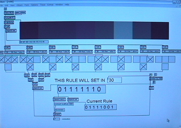
The piece as a whole can be thought of as being broken into a network of four software nodes, each with a specific function. The core node is reversible.py, which acts as the main program calculating the cellular automata. The rule which governs the CA is generated by rule.mxb, which takes input from a small camera and sends the new eight digit binary rule to reversible.py. The generational matrix of the CA’s history is presented on a flat screen display by history.mxb. Taking input from a DV cam, history.mxb simultaneously records the CA input as well as tracks positional change, sending the new seed data to reversible.py. Three BASICStampII microcontrollers run ser_out.bs2 each receiving their serial data from reversible.py and outputting it as high or low voltage to 66 LEDs each, making for a total of 198 individually controlled LEDs.
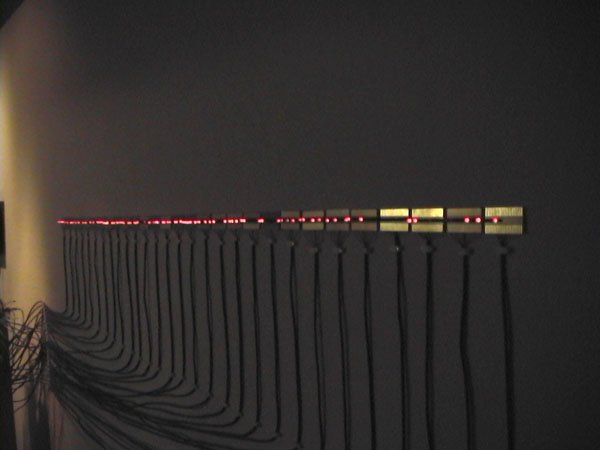
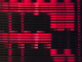
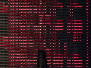
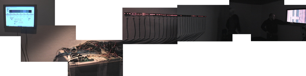
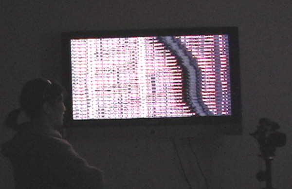
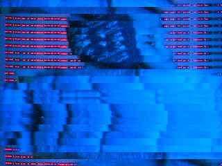
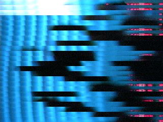
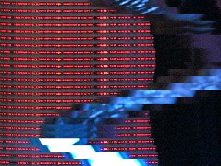
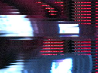
An array of 198 wall mounted LEDs display the current generation of the reversible cellular automata. Live cells are lit LEDs, dead cells are off. Mounted on the opposite wall is a 52-inch plasma flat screen monitor. Below it, a Cannon GL2 digital video camera is positioned on a tripod. The top of the camera’s view is focused on the line of LEDs on the opposing wall. The video from the camera is sent via Firewire into PC2 and captured by the Max/MSP application, history.mxb. Most of the image is cropped off, except for the very top. The resulting 720 X 20 matrix is a thin strip of video containing the real time display of the LEDs. Each of the previous 720 x 20 frames are placed one on top of the other to compose the final image. The most recent frame is placed at the bottom of the image and moves up 20 pixels when the next one is captured. Thus the current CA generation displayed by the LEDs is the bottom most layer of video, with the frames getting older the closer to the top they get. The resulting layered video displayed on the plasma screen thus follows the visual conventions of a classic one-dimensional cellular automata grid, with the Y-axis mapping generational history.
A smaller one-dimensional slice of 360 x 1 is also extracted from the original video by history.mxb. This array has the color red filtered out of it so that it does not pick up extraneous information from the LEDs themselves. It is then converted to grayscale and compared against itself. This comparison checks for change: pixels that differ from one frame to the next. The result is a binary array of pixels. The pixels are on if the original frames were different, off if not. It is then compressed to a 66 pixel array and the element number for each determinedly different pixel is sent via TCP connection to PC1 running reversible.py. When the data is received, reversible.py multiplies each element number by 3 to get the corresponding LED number and turns that LED on regardless of its current state.
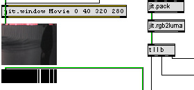
[history.mxb, motion track window]
With every new frame of video from the DV cam, history.mxb sends a signal over TCP to reversible.py to update the next generation of cellular automata. Running on PC1 the Python program reversible.py works as the central nervous system for the work. It is the main engine that runs the CAs as well as running as many of the extraneous calculations as possible. Given that Python takes less processor power than Max/MSP and has vastly more access to memory then the BASICStampIIs, I wanted reversible.py to do as much of the labor as possible.
Using Twisted, an event-driven networking framework, reversible.py communicates with both Max/MSP programs. All the automata calculations are done in the dataReceived() method, thus the CA runs only when it receives a new rule, new data, or just an “empty” update message. The incoming messages are tagged so that they can be sorted. A message starting with ‘r’ is a rule, an ‘n’ means nothing, (just update the next generation). Otherwise the numbers coming in represent cells born by human interaction. For the sake of speed, the manipulated cells are 1/3 res. The data integers are on a scale of 1 to 66 and must be multiplied by three after being received. The accuracy of interference is therefore off by plus or minus one cell. Each generation of cells is held as a binary integer list in Python. After the new generation of reversible Cellular Automata is calculated, the cells corresponding to the data received from history.mxb are born. If they were already alive, no change takes place. The data is then broken up into digestible pieces the BASICStampIIs can understand. The list holding the CA’s current generation is broken up into thirds and using pySerial each section is sent via USB to serial adaptor to its appropriate stamp. Ideally, one could just send a binary string of 1s and 0s; however, because each ASCII character is a byte, a string of 66 bytes exceeds the BASICStampII’s memory limit. This is upsetting since the list is only binary information. To get around this problem, every eight elements in the list are converted from binary to decimal which generates a number from 0 to 255. That number is then converted to its corresponding ASCII character. The ASCII set consists of 256 characters: every digit, every letter, big and small, every symbol on the keyboard and then some. Since the number 66 is not evenly divisible by 8, each stamp receives 8 encoded ASCII characters and two face value 1s and 0s. An input string consisting of only ten bytes is something that the stamps can handle.
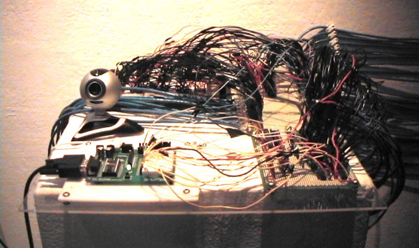
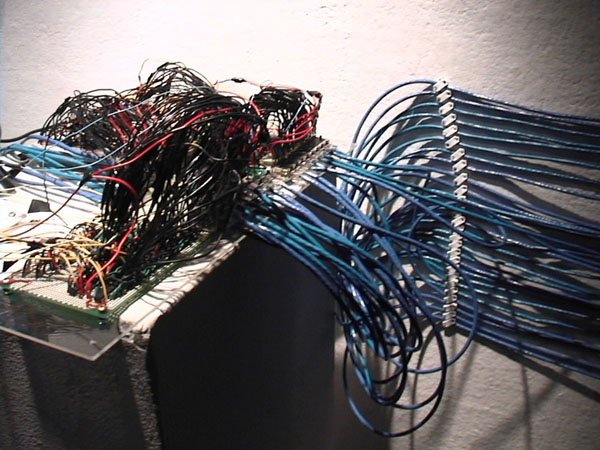
Three Parallax BasicstampII microcontrollers along with six 74HC164 chips and twenty-four 74HC374 chips handle the task of controlling the LEDs. Because each stamp only has 16 pins to be used as outputs, a massive system to increase the outputs had to be implemented. The solution was a circuit design adapted from the Microcontroller Application Cookbook by Matt Gilliland. This circuit utilizing one 74HC164 chip and four 74HC374 chips enabled me to get 32 outputs out of 7 pins on the stamp. The 74HC164 chip is an 8 bit ‘shift register’ which can receive serial data from a single I/O line and output the corresponding bits in parallel. I doubled up the output-expanding circuit design to get 64 output pins out of 14 on each stamp. For all three stamps I recreated this circuit six times total. The 2 pins on each stamp not used in the circuit output their signal directly. These three combined circuits, along with the three BASICStampIIs, make up the crisscrossed wire network displayed on the pedestal.
[This is circuit diagram is 1/3 of the entire circuit. It is repeated once for each of the 3 microcontrollers.]
The BASIC program, ser_out.bs2, runs on each of the stamps and has the task of converting the ASCII values to binary electrical signals for each LED. ser_out.bs2 receives a string of ten ASCII characters through the stamp’s serial port from PC1. The last two characters of the string are face value binary numbers and are sent directly to output pin 15 and 16 respectively. For the eight ASCII characters a for-loop is set up for the output expansion circuit. The loop runs four times, with the two circuits that run off of each chip being processed in parallel. Thus the first character in a string is processed in the same loop as the fifth. This is done in order to achieve a more parallel processing of the display sequence. In each loop iteration, the eight individual bits of the ASCII character are sent via output pins into the circuit’s eight bit shift register. The corresponding high and low voltages of the BASICStampIIs and the output-expansion circuits control the on and off states of the LEDs. A dead cell causes the corresponding LED to lose power; a live cell causes it to receive the electricity it needs to light.
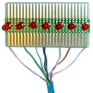
The wiring is somewhat the opposite of what might be expected. The output pins act as ground for the LEDs. This means that they all can share one positive line, but it also means zeros, low voltages from the outputs, turn them on. I resolved this problem by having reversible.py invert all the binary automata data after it is calculated but before it is sent to the microcontrollers. The LEDs are mounted to soldering plates. Each plate holds seven LEDs (except for the last one) and thus must have seven wires to the corresponding outputs plus one for positive. This made Cat5 cable, which has eight lines, the perfect modular hardware solution for wiring each wall mounted soldering plate. Female Ethernet connectors, each containing seven output lines and one positive line, are soldered to the main expansion circuit board. Each wall-mounted board of seven LEDs is soldered to a line of Cat5 cable with a male Ethernet plug on the other end. In total, 29 lines of Cat5 cable plug into the circuit, each responsible for 7 LEDs. The final resulting array of 198 wall mounted LEDs displays the current generation of the reversible cellular automata, and the cycle continues.
All the hardware and software elements come together to generate an environment which collides the ordinary lives of us Irreversible Automata with the digital “lives” of the Reversible Cellular Automata. Rather than a simple pixel-by-pixel display hermetically sealed in the other side of a screen, the cellular grid is constructed from the realtime digitization of the natural world. The computational loop is opened and extraneous visual data is allowed to seep in. Viewing the exposed hardware and the exposed rule system changes the very rule system being exposed. The Cellular Automata engage the viewer and the viewer intern engages the CA. The casualty-bound system and the non-causality-bound system merge into a single entity.
I am fascinated by the unanticipated viral fundamentals of causality’s true nature. Time, it seems, is inescapable. This is a disappointing, yet anticipated forgone conclusion. It is expected that no amount of mathematical manipulation of alternate computational systems, however similar, should be able to change the rules that fabricate time itself. The interesting part is not what happens to us, but what happens to them. Colliding a world of Irreversible Automata with a world of Reversible Automata results in a single irreversible world. We infect the Reversible Cellular Automata with our causality. We are not freed from the causality governing our system; rather, it is spread. The binary configuration of each generation of the reversible cellular automata in essence carries with it an embedded history. When that pattern is affected externally, it ceases to be reversible. The same steps to move forward must be applied to move backward. Due to our influence, the cells in the current generation are born regardless of the rule. The CA rule, however, did not determine our movements, and there is no way for us to run reality backwards in sync either. The reversible CA can only move back through time until the moment when it was last engaged by the natural world. One could argue that like most things they might have been “happier” if we left them alone.
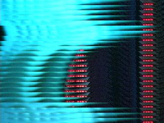

The human participants in the work are influenced just as strongly by the Reversible Automata but in a different manner altogether. Although we maintain our chronological restraints, we gain the opportunity to interact with a parallel computational world from within. Much like the Cellular Automata themselves, behavioral patterns emerge in the viewers as well. Participants most often begin by moving their whole body slowly, cautiously observing the forms they are creating with their silhouette on screen. They then begin to concentrate on particular motions, such as weaving arrangements with their hands to create helix patterns. Once viewers gain awareness of how the images are processed and the effects which they themselves have on the system, cautious movements give way to deliberate activities. I witnessed many participants timing movements to coincide with the rate of generational movement as to reconstruct images, like one’s face, in the CAs history. Quick and jittery hand gestures became frequently used to stir up the generational banding common in Reversible Cellular Automata. This would in turn seed more and more complex and interesting development in both worlds. Some human minds got extremely creative and began to manipulate the CA’s generational history with their own light sources from pocket electronic devices. Cellphone screens moved along the LED array were used to interfere with the light pattern capture. One participant began taking timed pictures in order to bleach out the LEDs with his flash one whole generation at time. Finally, some participants discovered that they could change the color of the LEDs background on screen as well as the whole ambient color of the room. The screen was bright enough that the camera picked up the light reflecting off the opposite wall. Any intense color, if left on camera long enough to fill up all the current frames of history would recursively begin filling the room with its light. Time and again fascination elicited emergent behavior that led to more fascination and more interaction. Once the interest was ignited, questions came that leaded to more contemplation and in turn, more questions.
The effects that CAs have on us proved to be thought provoking as well as mesmerizing. Because of this, I consider this project a truly successful work. My drive in creating this piece was not to make something at which one would take a single glance at and say “Oh I get it.” In the past, my work has often been a little too easily digestible for my liking. This piece was intentionally not so. I created a work that was instead poignant, conceptually far-fetched, and hard to digest at first glance. Art that is spoon-fed to the community quickly becomes as dull as it is popular. In trying to get as far from that as possible, I also created something that became incredibly difficult to explain in one sitting. It is not necessary to understand everything there is to know about Cellular Automata and ontologies for reality to enjoy the natural computation of our world. Neither is it necessary to completely understand every element of the piece to simply enjoy it. As mathematics gives way to philosophy, there is no understanding it all. The purpose of the piece is to act as a catalyst for the participants’ own thought trains. This computation is Class Four, it does not stop at a particular quantifiable result.
Rucker, Rudy. 2005. The Lifebox the Seashell and the Soul. New York: Thunder’s Mouth Press.
Wolfram, Stephen. 2002. A New Kind of Science. Wolfram Media.
Fuller, Mathew. 2005. Media Ecologies. Cambridge, MA: MIT Press.
Stork, David G. 1996. HAL's Legacy: 2001's Computer as Dream and Reality. Cambridge, MA:
MIT Press.
Wikipedia, The Free Encyclopedia. 2003. Cellular Automaton.
http://en.wikipedia.org/wiki/Cellular_automata (accessed Jan 2006)
Gilliland, Matt. 2000. The Microcontroller Cookbook. Woodglen Press
Exhibitions
- Oath
- 127 BPM
- Red White & Blue
- Future Flower
- Vicious Virus Versus
- Litewall Games
- V2V
- Not a Hero
- DPS
- Spectacle & Lament
- MFA Prep Course
- MKDDR
- /hug
- A Language 4 the People
- Media - Me
- Bombs ¬ROMs
- Looks Very Tidy
- Tool Shed Days
- Buildup
- slow progress for democracy
- Seed
- Scrapper and Mixmaster
- Karaoke Ice
- Combat! Client
- Sticky Anonymity
- Rev./Irrev. Automata
- Prototype: OmniVision
- 24-Hour Surveillance
- Chicken
- Polyphonic Peelings
- n0easyAnswersThisTime
- Any3Letters.Com
- Spread